Logistic Regression

The solution to a classification problem is a prediction of some independent variables’ class from a finite number of labels, rather than a real-valued output as in linear regression. In the case of binary classification, a classification problem with two classes, logistic regression can be used to fit a statistical model’s parameters to an observed distribution.

Initialisation

A handful of modules and convenience functions are required for the subsequent examples.

import matplotlib as mpl
import matplotlib.pyplot as plt
from matplotlib.ticker import (MultipleLocator, AutoMinorLocator, FormatStrFormatter)
import numpy as np
import sklearn.datasets
import math
%matplotlib inline

def new_plot():
    fig = plt.figure(dpi=300)
    ax = fig.add_subplot(1,1,1)
    ax.set_xticks([])
    ax.set_yticks([])
    ax.set_aspect('auto')
    return fig, ax

Logistic Function

The sigmoid or logistic function returns a value in the interval \((0,1)\) and is defined:

\[\sigma(u) = \dfrac{1}{1+e^{-u}}\]

The inverse of the logistic function is the logit or log-odds function for some observation according to a probability distribution:

\[\sigma^{-1}(u) = \log\left(\dfrac{p}{1-p}\right)\]

The sigmoid function, in code:

def sigmoid(u):
    return 1 / (1+math.e ** -u)

The sigmoid function, visualised:

x = np.linspace(-8, 8, 1000)
f, ax = new_plot()
ax.set_xticks([])
ax.yaxis.set_major_locator(MultipleLocator(1))
ax.grid()
ax.plot(x, sigmoid(10 * x), 'green', label="10x")
ax.plot(x, sigmoid(2 * x), 'red', label="2x")
ax.plot(x, sigmoid(x), label="x")
ax.legend(loc='lower right')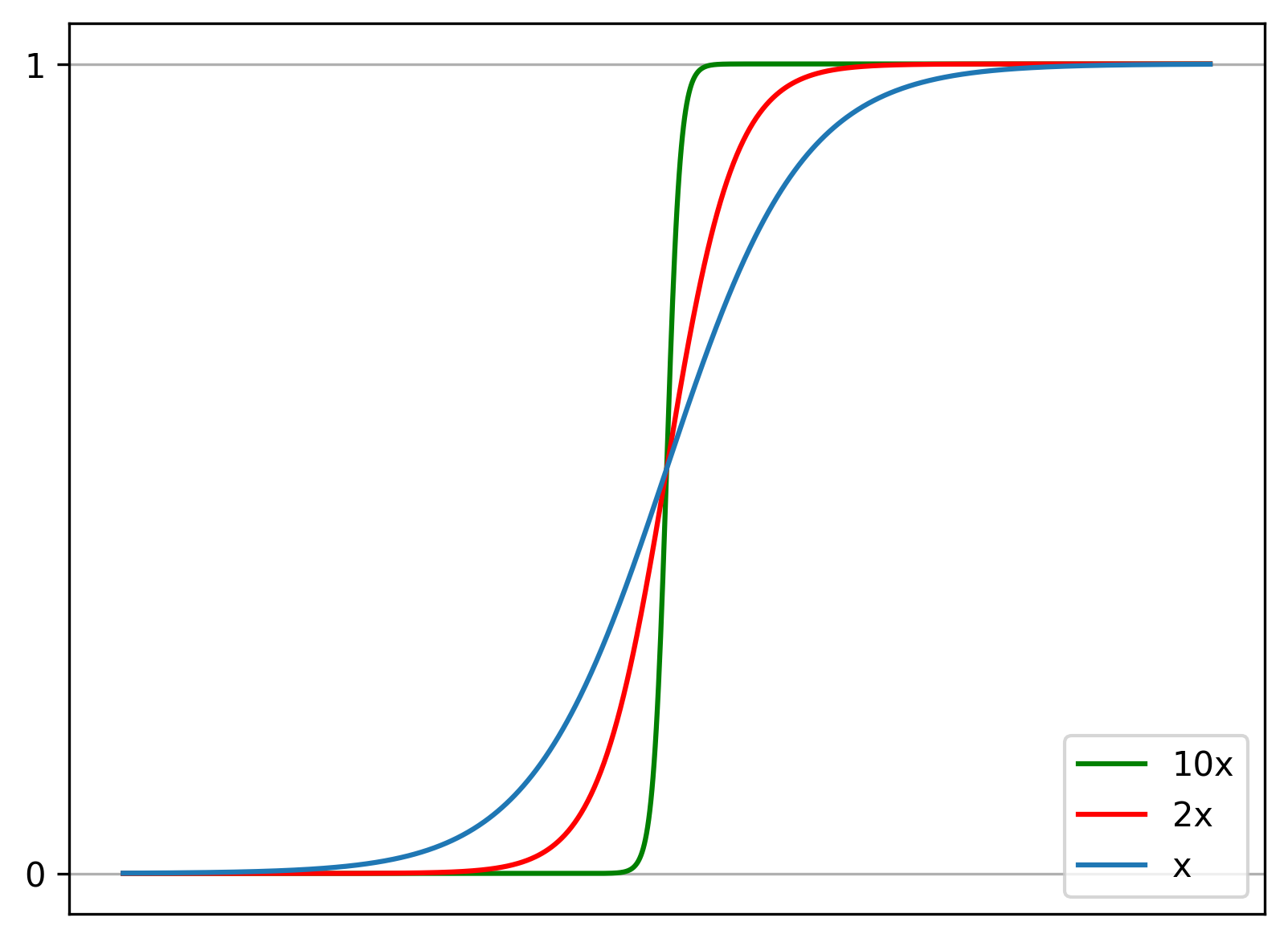

Principles of Logistic Regression

Logistic regression models the log-odds of a binary outcome in a Bernoulli distribution as a linear combination of the independent variable. Consequently, the probability that the random variable \(Y\) takes the value \(1\) is the application of the logistic function to this linear combination.

\[p = P(Y = 1)\]

\[\log\left(\dfrac{p}{1-p}\right) = w_0x_0 + w_1x_1 + \ldots + w_nx_n\]

\[\mathbf{w} = \langle w_0, w_1 \ldots w_n \rangle\]

\[\mathbf{x} = \langle x_0 = 1, x_1 \ldots x_n \rangle\]

\[P(Y=1|\mathbf{w},\mathbf{x}) = \sigma(\mathbf{w}^T\mathbf{x})\]

\[P(Y=1|\mathbf{w},\mathbf{x}) = h_{\mathbf{w}}(\mathbf{x})\]

In this binary classification problem, the model \(h_{\mathbf{w}}(\mathbf{x})\) is the linear function \(\mathbf{w}\cdot\mathbf{x}\) passed through a threshold function, returning a probability that can be converted to the dependent variables’ classification via a random variable, rather than a real value as in regression. This linear function is called the decision boundary or linear separator. A data set admitting a linear separator is considered linearly separable and there exists a solution to the function \(h\) with zero cost. If the data set is linearly separable, the percepton learning rule for each element \(w_i\), \(x_i\) of \(\mathbf{w}\), \(\mathbf{x}\) will converge on an exact solution.

\[w_i \leftarrow w_i - \alpha (h_{\mathbf{w}}(\mathbf{x}) - y) \times x_{i}\]

Maximum Likelihood Estimation

Given a model with parameters \(\mathbf{w}\), a cost function must be provided to quantify the error of the current model. Likelihood is a function of the parameters of a model (in this case, \(\mathbf{w}\)) measuring the probability of the observed data occurring under that model.

\[\mathcal{L}(\mathbf{w} | y; \mathbf{x}) = P(Y = y | \mathbf{w},\mathbf{x})\]

As the logistic regression problem is known to follow a Bernoulli distribution, the probability mass function for each outcome \(y\) of the random variable \(Y\) is:

\[ P(Y = y | \mathbf{w},\mathbf{x}) = \begin{cases} h_{\mathbf{w}}(\mathbf{x}) & \text{if } y = 1 \\ 1-h_{\mathbf{w}}(\mathbf{x}) & \text{if } y = 0 \end{cases} \]

This can be expressed in a single expression as:

\[P(Y = y | \mathbf{w},\mathbf{x}) = h_{\mathbf{w}}(\mathbf{x})^y (1-h_{\mathbf{w}}(\mathbf{x}))^{1-y}\]

Maximising this value, the likelihood, will fit the model to the observations, through it is more common to minimise the negative log-likelihood, given by:

\[ L(\mathbf{w}) = -(y\log(h_{\mathbf{w}}(\mathbf{x})) + (1-y)\log(1-h_{\mathbf{w}}(\mathbf{x}))) \]

The average cost over many examples:

\[L(\mathbf{w}) = -\frac{1}{N}\sum_n^N (y_{n}\log(h_{\mathbf{w}}(\mathbf{x}_n)) + (1-y_n)\log(1-h_{\mathbf{w}}(\mathbf{x}_n)))\]

The derivative of the cross-entropy cost function:

\[\nabla L(\mathbf{w}) = -\frac{1}{N}\sum_n^N (y_{n} - h_{\mathbf{w}}(\mathbf{x}_n))\times \mathbf{x}_n\]

The weight update rule for each \(w\) in \(\mathbf{w}\):

\[w_i \leftarrow w_i + \alpha\sum_n^N (y_{n} - h_{\mathbf{w}}(\mathbf{x}_n))\times x_{n,i}\]

With theses expressions, it is possible to perform logistic regression, and update the weights of the underlying function to redraw the decision boundary.

def create_minibatches(a, m):
    n = int(x.shape[0] / m)
    return np.array_split(a[:m * n], n), n

def h(W, X):
    return sigmoid(sum(W * X))


def logistic_regression(a, m, W, y, X):
    X = np.concatenate((np.ones((X.shape[0],1), dtype=int), X), axis=1)
    X, n = create_minibatches(X, m)
    y, n = create_minibatches(y, m)
    for b in range(n):
        for w in range(W.size):
            W[w] += a * sum([((h(W, X[b][x])) - y[b][x]) * X[b][x][w] for x in range(X[b].shape[0])])
    return W

In this example, the points are labelled in advanced (logistic regression is always a supervised problem). The decision boundary is drawn between the two classes. Note that this example is not linearly separable as the cost on the training set is not \(0\); it is a fairly good predictor, however.

X, y = sklearn.datasets.make_classification(n_samples=200,
                                            n_features=2,
                                            n_redundant=0,
                                            n_informative=1,
                                            n_clusters_per_class=1)
W = np.array([0.,0.,0.])
for _ in range(10):
    W = logistic_regression(0.001, 10, W, y, X)

f, ax = new_plot()
colors = ["blue", "red"]
ax.scatter(X[:, 0], X[:, 1],
           marker=".", c=y, s=1,
           cmap=mpl.colors.ListedColormap(colors))
ax.plot(X[:, 0],
        [X[i, 0] * (W[1] / (-1 * W[2]))
                  + W[0] for i in range(X.shape[0])],
        'green')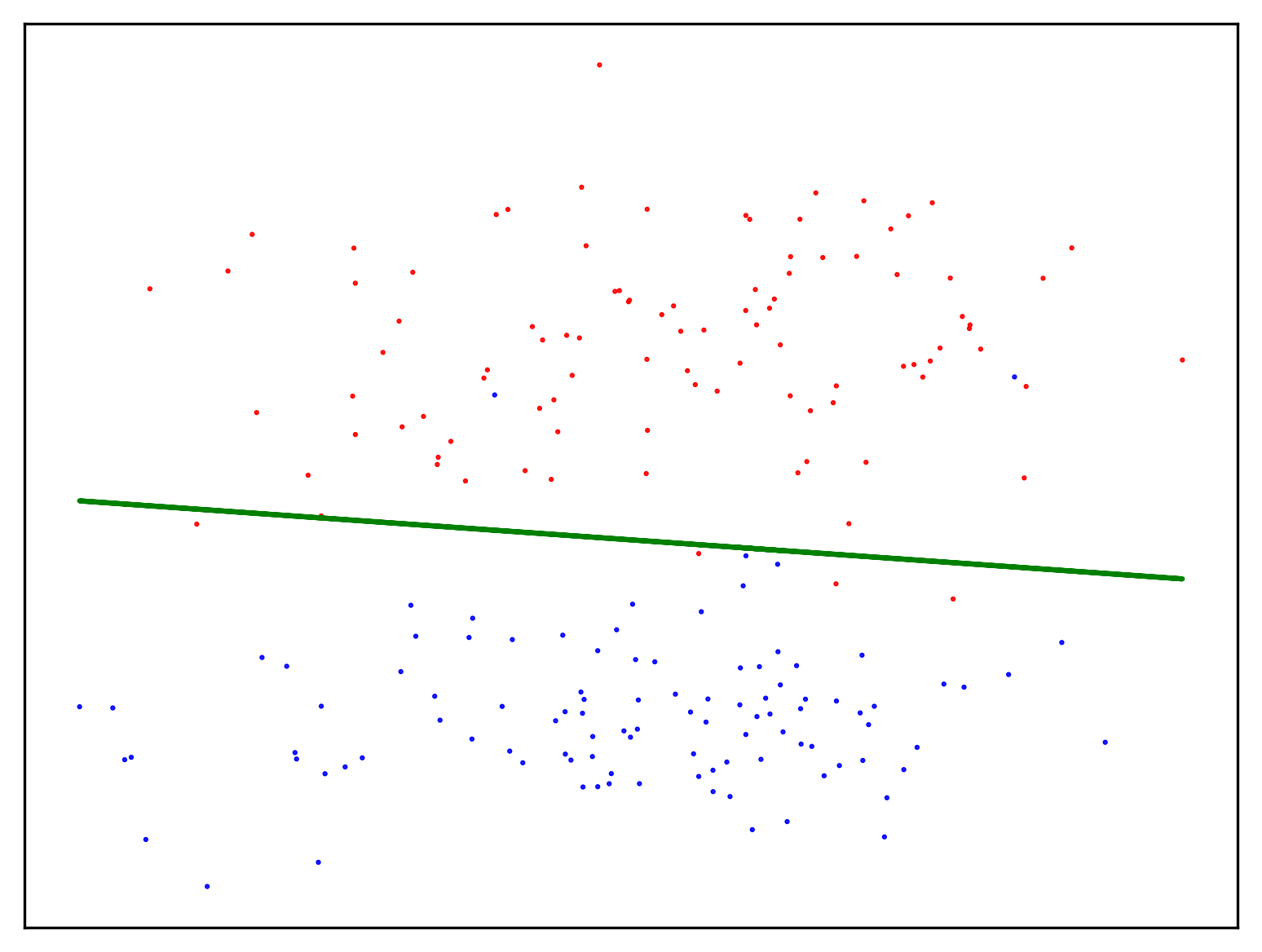

See Also

• Introduction to AI
• Linear Regression
• Logistic Regression
• Optimisation Algorithms
• Unsupervised Learning

Or return to the index.