Optimisation Algorhtims

Optimisation algorithms search for the optimal or, failing that, a good solution to a problem, all the while satisfying constraints. The optimal solution to a problem may be prohibitively difficult to calculate exactly, in which case an optimisation algorithm will attempt to improve upon a candidate solution.

Initialisation

A handful of modules and convenience functions are required for the subsequent examples.

import matplotlib as mpl
import matplotlib.pyplot as plt
import matplotlib.animation as animation
from matplotlib.ticker import (MultipleLocator, AutoMinorLocator, FormatStrFormatter)
import numpy as np
import sklearn.datasets
import math
import random
%matplotlib inline

def new_plot():
    fig = plt.figure(dpi=300)
    ax = fig.add_subplot(1,1,1)
    ax.set_xticks([])
    ax.set_yticks([])
    ax.set_aspect('auto')
    return fig, ax

Hill Climbing

A very simple optimisation algorithm is hill climbing. The process resembles generating neighbour solutions, which are close to the current solution, and moving in the direction of the best neighbour. This approach will rapidly converge on a nearby optima, however it is not guaranteed to find the global maxima - it is sub-optimal. Hill climbing is said to be greedy, it always takes the best quality neighbour at every step, even if a better solution can be reached by temporarily accepting a worse neighbour. The hill climbing implementation given here is made complicated by the animation code (which is written poorly).

def get_neighbours(x):
    return x + 1, x - 1


def init_hill_climbing():
    current = ax.scatter([], [], c='orange', zorder=5, s=100)
    equal = ax.scatter([], [], c='orange', zorder=5, s=100)
    better = ax.scatter([], [], c='green', zorder=5, s=100)
    worse = ax.scatter([], [], c='red', zorder=5, s=100)
    solution = ax.scatter([], [], c='green', zorder=5, s=100)
    converged = False
    return current, [better, equal, worse], solution, converged


def hill_climb(step):
    global converged
    global current_solution
    if step % 2 == 0:
        for plot in neighbour_plots:
            plot.set_visible(False)
        if converged:
            current_plot.set_visible(False)
            solution_plot.set_offsets([current_solution, f(current_solution)])
        else:
            current_plot.set_offsets([current_solution, f(current_solution)])
    else:
        local_neighbours = get_neighbours(current_solution)
        local_neighbour_solutions = [f(i) for i in local_neighbours]
        local_neighbour_quality = [[],[],[]]

        for i in range(2):
            if local_neighbour_solutions[i] > f(current_solution):
                local_neighbour_quality[0].append(local_neighbours[i])
            elif local_neighbour_solutions[i] == f(current_solution):
                local_neighbour_quality[1].append(local_neighbours[i])
            else:
                local_neighbour_quality[2].append(local_neighbours[i])

        for i in range(3):
            if len(local_neighbour_quality[i]) > 0:
                neighbour_plots[i].set_visible(True)
                neighbour_plots[i].set_offsets(np.stack([local_neighbour_quality[i],
                                                         f(np.array(local_neighbour_quality[i]))]).T)

        if max(local_neighbour_solutions) > f(current_solution):
            current_solution = local_neighbours[local_neighbour_solutions.index(max(local_neighbour_solutions))]
        else:
            converged = True

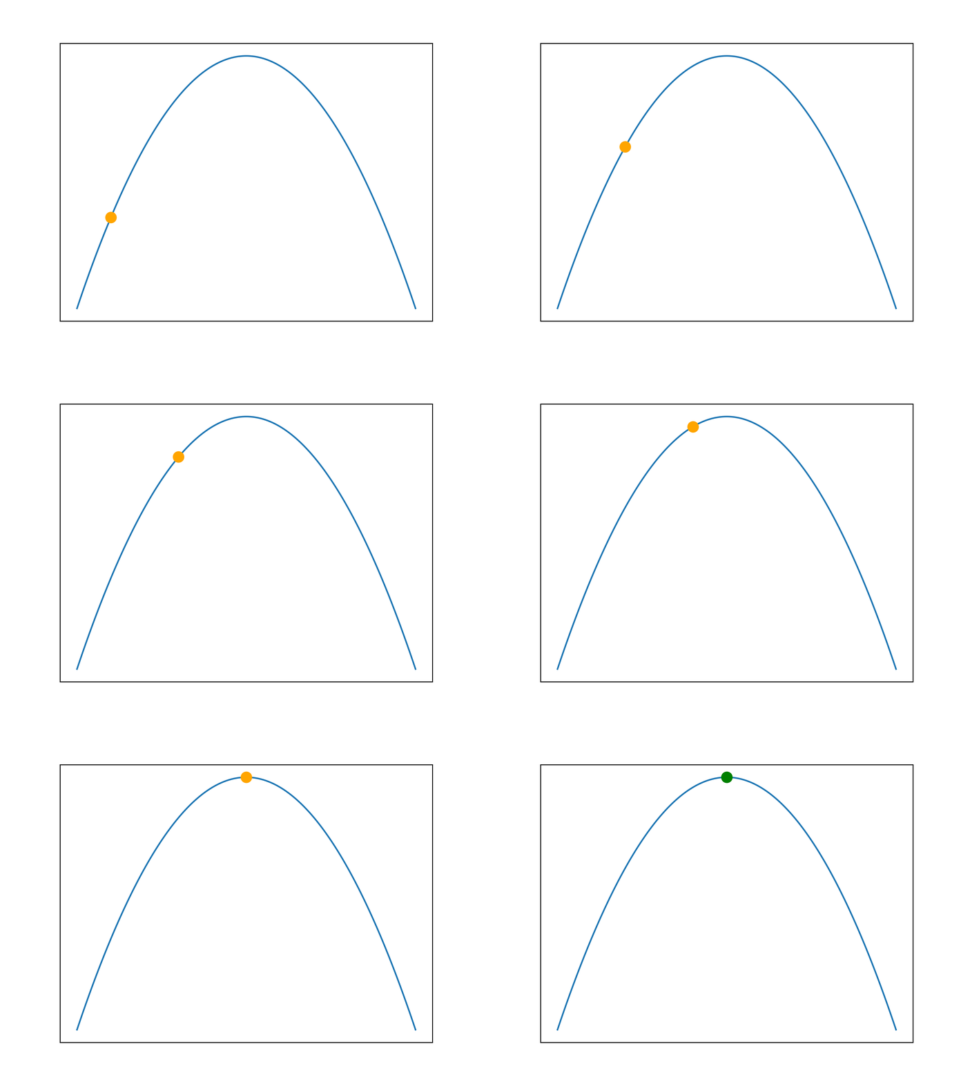
For functions with a single maxima, hill climbing finds the optimal solution.

def f(x):
    return -x**2


x = np.linspace(-5, 5, 1000)
fig, ax = new_plot()
ax.plot(x, f(x))

current_plot, neighbour_plots, solution_plot, converged = init_hill_climbing()
current_solution = -4

anim = animation.FuncAnimation(fig=fig, func=hill_climb, frames=11, interval=500)
anim.save('../../animations/optimal.gif')

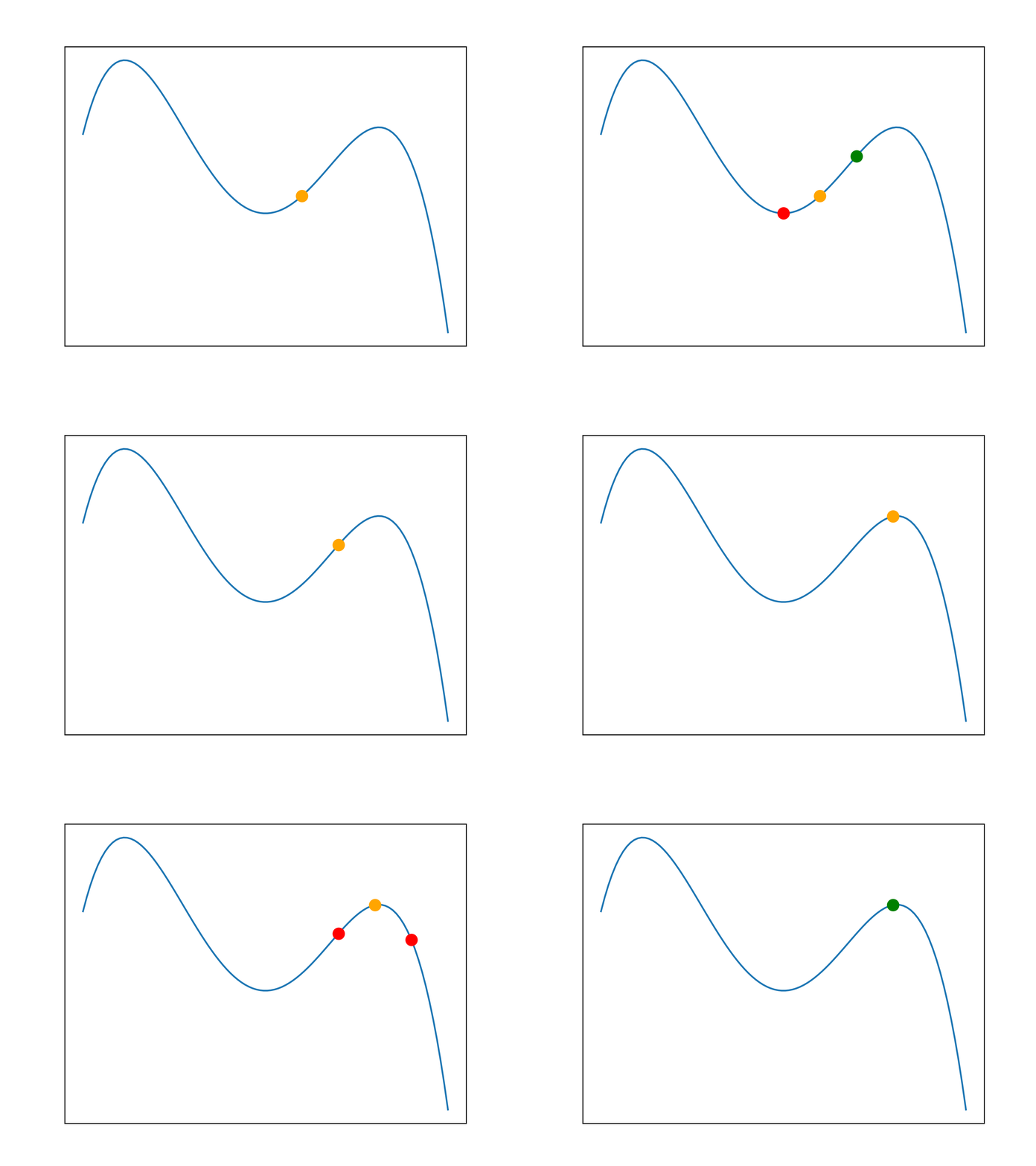
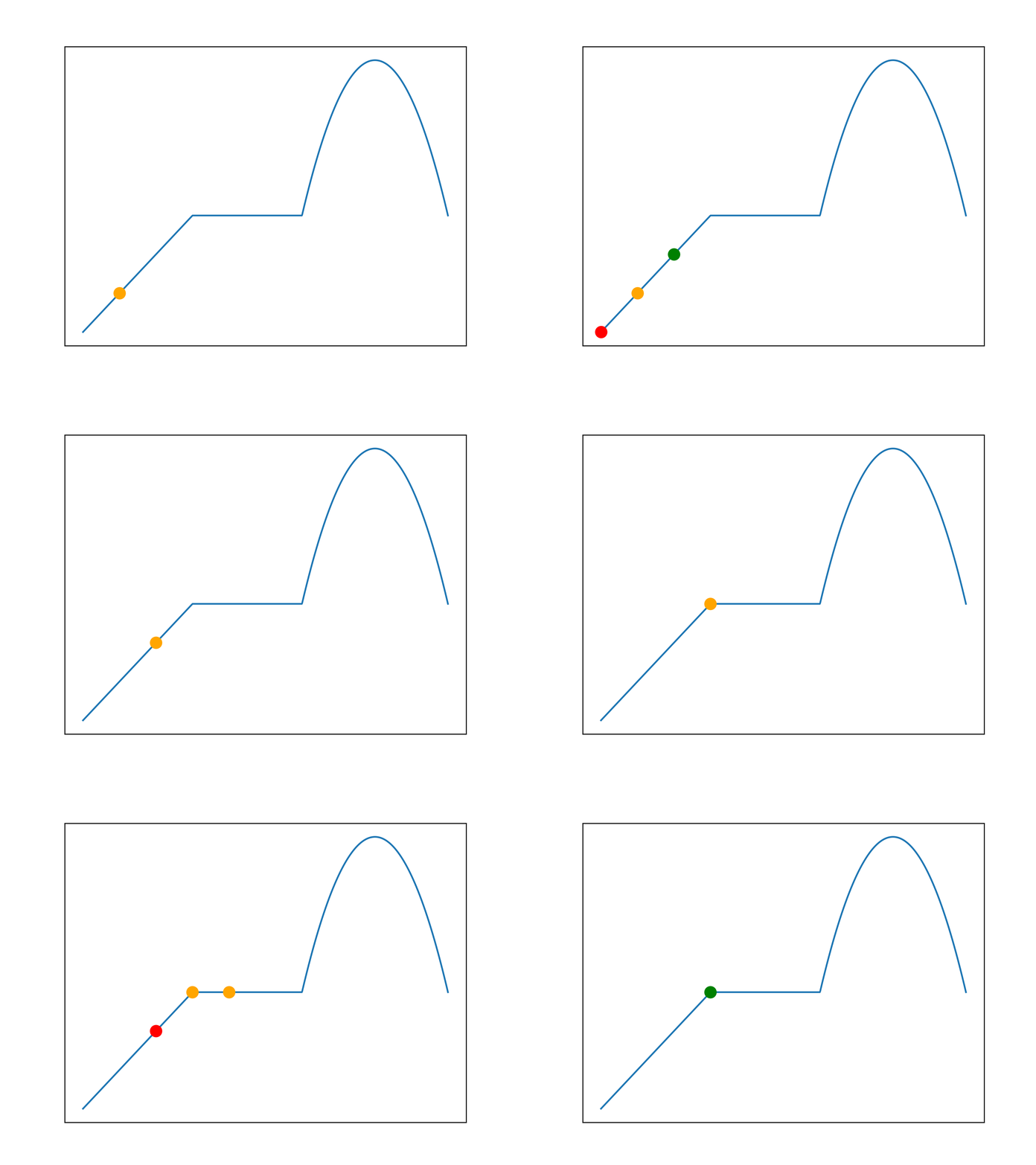
Applied to more complicated problems, hill climbing may not find a perfect solution as it can become trapped in a local maxima. It is unable to traverse the search space to find better solutions. Sometimes this is not a problem, as a sub-optimal solution may be adequate. The following examples illustrate this problem.

def f(x):
    return (-x**4 - x**3 + 24*x**2)


x = np.linspace(-5, 5, 100)
fig, ax = new_plot()
ax.plot(x, f(x))

current_plot, neighbour_plots, solution_plot, converged = init_hill_climbing()
current_solution = 1

anim = animation.FuncAnimation(fig=fig, func=hill_climb, frames=7, interval=500)
anim.save('../../animations/local_maxima.gif')

def f(x):
    def _f(x):
        if x < 3:
            return x
        elif x < 6:
            return 3
        else:
            return -(x-8)**2+7

    return np.vectorize(_f)(x)

x = np.linspace(0, 10, 1000)
y = [f(x) for x in x]
fig, ax = new_plot()
ax.plot(x, y)

current_plot, neighbour_plots, solution_plot, converged = init_hill_climbing()
current_solution = 1

anim = animation.FuncAnimation(fig=fig, func=hill_climb, frames=7, interval=500)
anim.save('../../animations/plateau.gif')

Simulated Annealing

Simulated annealing is one strategy to improve the performance of hill climbing algorithms.

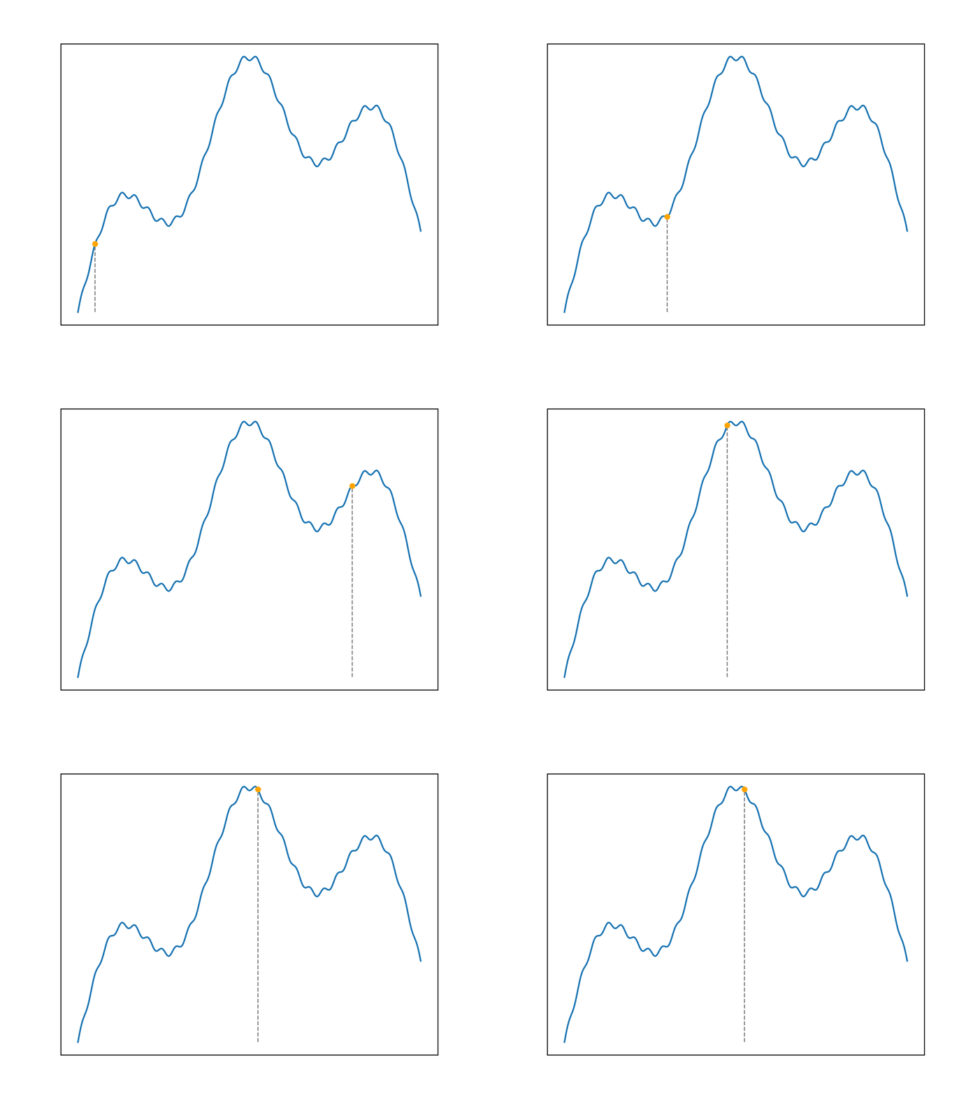
At each step, a random neighbour solution is generated. If this candidate solution is better than the current one, it is immediately selected. If the generated neighbour is worse, it is accepted with some probability. This probability is inversely proportional to how bad this neighbour is (less bad neighbours are more likely to be accepted). Over time, this probability is decreased according to the schedule. This is called the annealing process.

Initially, the annealing algorithm is likely to accept a series of worse neighbours, allowing it to escape a local maxima and traverse the search space. The algorithm gradually forms a basis of attraction to increasingly small sections of the search space which contain a maxima.

Because of the random nature of annealing, the algorithm is not optimal, however the probability of locating the global maxima approaches 1 as the annealing schedule is extended. Brute-force examination of the search space may be faster than random annealing in some cases. Often, the annealing approach is likely to improve upon a solution quickly, by escaping several local optima.

def update_temperature(T):
    return 0.999*T


def p_worse_neighbour(c, n, T):
    return math.e**((f(n) - f(c))/T)


def get_random_neighbour(x):
    if random.randint(0,1):
        return x + 4 if x + 4 < 160 else x - 4
    else:
        return x - 4 if x - 4 > 0 else x + 4


def simulated_annealing():
    global current_solution
    global T
    neighbour = get_random_neighbour(current_solution)
    if f(neighbour) <= f(current_solution):
        if p_worse_neighbour(current_solution, neighbour, T) > random.random():
            current_solution = neighbour
    else:
        current_solution = neighbour
    T = update_temperature(T)

Define the search space, the starting solution and the initial temperature.

def f(x):
    return 0.4*(2*math.sin(0.5*x) + 20*math.sin(0.1*x) + 80*math.sin(1/60*x))

x = np.linspace(0, 170, 1000)
current_solution = 12
T = 20

Put together an animation of the annealing process.

fig, ax = new_plot()

ax.plot(x, np.vectorize(f)(x), zorder=2)
current = ax.scatter([], [], c='orange', zorder=3, s=20)
line, = ax.plot([], [], c='gray', ls='--', zorder=1, lw=1)

def animate_simulated_annealing(frame):
    global current_solution
    global T
    simulated_annealing()
    current.set_offsets([current_solution, f(current_solution)])
    line.set_xdata([current_solution, current_solution])
    line.set_ydata([0, f(current_solution)])

anim = animation.FuncAnimation(fig=fig,
                               func=animate_simulated_annealing,
                               frames=2000, interval=20)
anim.save('../../animations/simulated_annealing.gif')

See Also

• Introduction to AI
• Linear Regression
• Logistic Regression
• Optimisation Algorithms
• Unsupervised Learning

Or return to the index.